|
|
Simple Linear Regression
Generating the Model
Fitting data with a simple linear regression can be performed via the lm function. In order to view the results of the fit, a user must use the summary function. fit = lm (ResponseVariable ~ PredictorVariable, data = ElementName) summary( fit ) Example: > fit = lm (bp ~ pres, data = forbes) > summary ( fit ) 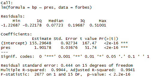
Viewing Diagnostic Plots
The common diagnostic plots can be viewed by plotting the fit result. The user can display all four diagnostic plots at once by defining a layout scheme. fit = lm (ResponseVariable ~ PredictorVariable, data = ElementName) layout ( matrix ( c( 1,2,3,4 ), 2, 2 )) plot ( fit ) Example: > fit = lm (bp ~ pres, data = forbes) > layout ( matrix( c( 1,2,3,4 ), 2, 2 )) > plot ( fit ) 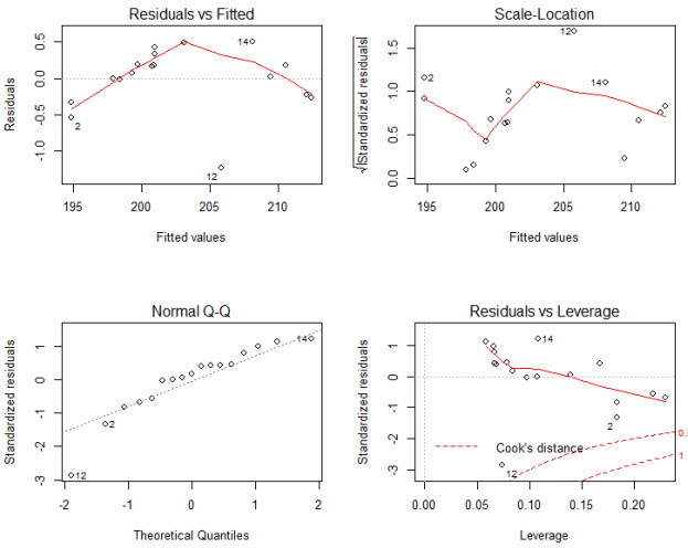
Viewing Model Coefficients
Model coefficients can be viewed via the coefficients function. fit = lm (ResponseVariable ~ PredictorVariable, data = ElementName) coefficients ( fit ) Example: > fit = lm (bp ~ pres, data = forbes) > coefficients ( fit ) 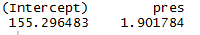
Viewing Confidence Intervals for Model Parameters
The confidence intervals for the model parameters can be viewed via the confint function. fit = lm (ResponseVariable ~ PredictorVariable, data = ElementName) confint (fit , level = ConfidenceLevel ) Example: > fit = lm (bp ~ pres, data = forbes) > confint ( fit , level = 0.95) 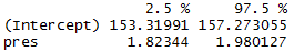
Viewing Predicted Fit Values
The fitted values can be viewed via the fitted function. fit = lm (ResponseVariable ~ PredictorVariable, data = ElementName) fitted ( fit ) Example: > fit = lm (bp ~ pres, data = forbes) > fitted ( fit ) 
Viewing Residuals
The residuals can be viewed via the residuals function. fit = lm (ResponseVariable ~ PredictorVariable, data = ElementName) residuals ( fit ) Example: > fit = lm (bp ~ pres, data = forbes) > residuals ( fit ) 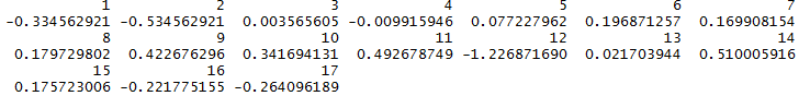
Viewing ANOVA Table
The ANOVA table can be viewed via the anova function. fit = lm (ResponseVariable ~ PredictorVariable, data = ElementName) anova ( fit ) Example: > fit = lm (bp ~ pres, data = forbes) > anova ( fit ) 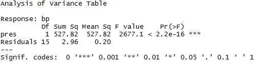
Viewing Covariance Matrix for Model Parameters
The covariance matrix can be viewed via the vcov function. fit = lm (ResponseVariable ~ PredictorVariable, data = ElementName) vcov ( fit ) Example: > fit = lm (bp ~ pres, data = forbes) > vcov ( fit ) 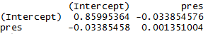
|
