Multiple Regression

---

Generating the Model
Fitting data with a multiple regression can be performed via the lm function. In order to view the results of the fit, a user must use the summary function. 

fit = lm (ResponseVariable ~ PredictorVariable1 + Predictor Variable2 + PredictorVariable3 ... ,  data = ElementName)
summary( fit )

Example:
> fit = lm (stack.loss ~ Air.Flow + Water.Temp + Acid.Conc., data = stackloss) 
> summary ( fit )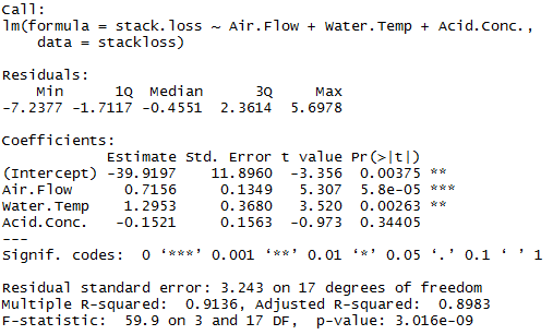

---

Viewing Diagnostic Plots
The common diagnostic plots can be viewed by plotting the fit result. The user can display all four diagnostic plots at once by defining a layout scheme. 

fit = lm (ResponseVariable ~ PredictorVariable1 + Predictor Variable2 + PredictorVariable3 ... ,  data = ElementName)
layout ( matrix ( c( 1,2,3,4 ), 2, 2 ))
plot ( fit )

Example:
> fit = lm (stack.loss ~ Air.Flow + Water.Temp + Acid.Conc., data = stackloss) 
> layout ( matrix( c( 1,2,3,4 ), 2, 2 ))
> plot ( fit )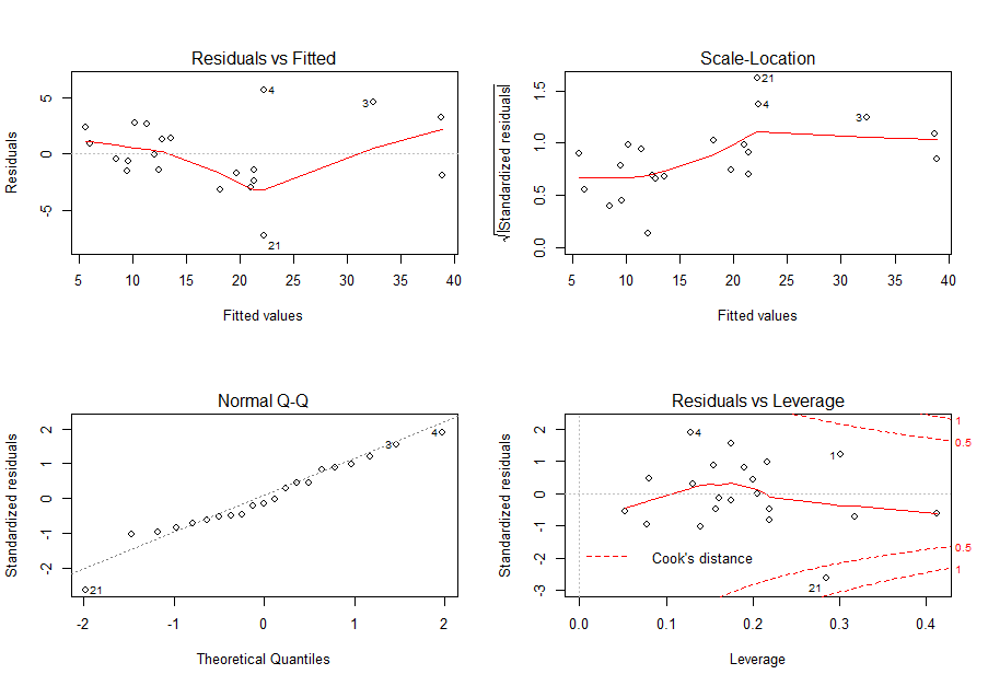

---

Viewing Model Coefficients
Model coefficients can be viewed via the coefficients function. 

fit = lm (ResponseVariable ~ PredictorVariable1 + Predictor Variable2 + PredictorVariable3 ... ,  data = ElementName)
coefficients ( fit )

Example:
> fit = lm (stack.loss ~ Air.Flow + Water.Temp + Acid.Conc., data = stackloss) 
> coefficients ( fit )

---

Viewing Confidence Intervals for Model Parameters
The confidence intervals for the model parameters can be viewed via the confint function. 

fit = lm (ResponseVariable ~ PredictorVariable1 + Predictor Variable2 + PredictorVariable3 ... ,  data = ElementName)
confint (fit , level = ConfidenceLevel )

Example:
> fit = lm (stack.loss ~ Air.Flow + Water.Temp + Acid.Conc., data = stackloss) 
> confint ( fit , level = 0.95)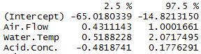

---

Viewing Predicted Fit Values
The fitted values can be viewed via the fitted function.

fit = lm (ResponseVariable ~ PredictorVariable1 + Predictor Variable2 + PredictorVariable3 ... ,  data = ElementName)
fitted ( fit )

Example:
> fit = lm (stack.loss ~ Air.Flow + Water.Temp + Acid.Conc., data = stackloss) 
> fitted ( fit )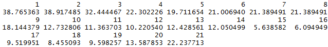

---

Viewing Residuals
The residuals can be viewed via the residuals function. 

fit = lm (ResponseVariable ~ PredictorVariable1 + Predictor Variable2 + PredictorVariable3 ... ,  data = ElementName)
residuals ( fit )

Example:
> fit = lm (stack.loss ~ Air.Flow + Water.Temp + Acid.Conc., data = stackloss) 
> residuals ( fit )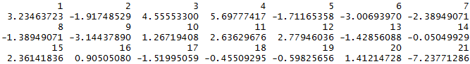

---

Viewing ANOVA Table
The ANOVA table can be viewed via the anova function. 

fit = lm (ResponseVariable ~ PredictorVariable1 + Predictor Variable2 + PredictorVariable3 ... ,  data = ElementName)
anova ( fit )

Example:
> fit = lm (stack.loss ~ Air.Flow + Water.Temp + Acid.Conc., data = stackloss) 
> anova ( fit )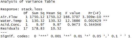

---

Viewing Covariance Matrix for Model Parameters 
The covariance matrix can be viewed via the vcov function. 

fit = lm (ResponseVariable ~ PredictorVariable1 + Predictor Variable2 + PredictorVariable3 ... ,  data = ElementName)
vcov ( fit )

Example:
> fit = lm (stack.loss ~ Air.Flow + Water.Temp + Acid.Conc., data = stackloss) 
> vcov ( fit )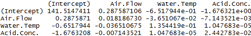

---

Assessing Relative Importance of each Predictor Variable
The relative importance of each predictor variable can be assessed via the functions available in the relaimpo package. 

fit = lm (ResponseVariable ~ PredictorVariable1 + Predictor Variable2 + PredictorVariable3 ... ,  data = ElementName)
install.packages ( "relaimpo" )
library ( relaimpo )
Relimp =  boot.relimp ( fit , type = "lmg"  , rela = TRUE)
plot ( booteval.relimp ( Relimp , sort = TRUE ))

Example:
> fit = lm (stack.loss ~ Air.Flow + Water.Temp + Acid.Conc., data = stackloss) 
> install.packages ( "relaimpo" )
> library ( relaimpo )
> Relimp =  boot.relimp ( fit , type = "lmg"  , rela = TRUE)
> plot ( booteval.relimp ( Relimp , sort = TRUE ))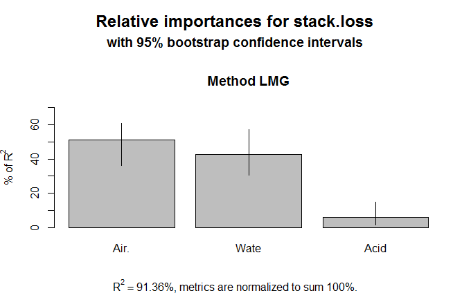

---